
I recently read the paper Lattice Convolutional Neural Network Modeling of Adsorbate Coverage Effects. The code for this paper was released on GitHub at https://github.com/VlachosGroup/lcnn
This paper advances the study of coverage effects (also called lateral interactions), by using deep learning methods to effectively model the physics of such interactions. The work applies this in particular to the study of adsorption, with the goal of predicting the energies and configuration of surface adsorbates.
A Brief Introduction to Adsorption
Before we go deeper into this paper, it might be useful to take a digression and discuss adsorption in more depth. Generally speaking, adsorption is the adhesion of molecules from a gas or liquid or dissolved solid onto a surface. Why does adsorption happen? It’s a phenomenon similar to surface tension in some ways. Note that the surface of a solid must be more energetically disfavorable than the interior, for otherwise it would be energetically favorable for the solid to break apart to create more surfaces. The surface energy characterizes the amount of energy required to create a surface. Returning to adsorption, the energetically disfavorable nature of the surface means that there’s opportunities for surface atoms to form chemical bonds with other atoms (which are called adsorbates). Adsorption turns out to be important in many applications such as catalyst and semiconductor design, so there’s a rich literature modeling adsorption from the materials science community.
Let’s introduce a couple of useful bits of terminology. An adsorption site is a location on the surface where an adsorbate can bond to the surface. The surface coverage (typically denoted \theta) is the fraction of the adsorption sites that are occupied. If there are multiple adsorbates, \theta_j is the fraction occupied by the j-th adsorbate.
One of the challenges of mathematically modeling an interesting adsorption system is that the adsorbates can interact with one another, creating “coverage effects.” For a large lattice with many adsorption sites, this can create fearsome multibody interaction effects that aren’t easy to model. To help you visualize this a bit better, let’s discuss the particular physical system that the current paper considers (I pulled the figure below from another reference)
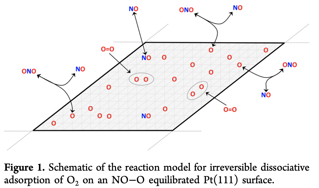
Note how there are many different adsorbates on the surface. It’s easy to imagine how this quickly turns into a challenging multibody physics problem. Here’s the chemical interaction that’s happening in the process of adsorption.
\textrm{Pt} + \frac{n_{\textrm{O}}}{2}\textrm{O}_2 + n_{\textrm{NO}} \to \textrm{O}_{\theta_{\textrm{O}}}\textrm{NO}_{\theta_{\textrm{O}}}/\textrm{Pt}
It’ll be useful to describe some mathematical conventions before we dive into the methods for this paper. A system with N sites and M different types of adsorbates is represented by a configuration vector \sigma of length N. Element i represents the occupancy of site i using the Ising convention, so
\sigma_i \in {\pm m, \pm (m-1), \dotsc, \pm 1, 0} where M = 2m or 2m+1
Computational Methods for Studying Adsorption Effects
Studying coverage effects computationally using density functional theory, is impractical due to the large numbers of degrees of freedom (DFT struggles for systems with more than 100 atoms in general). An interesting lattice might contain on the order of a 1000 sites, so DFT calculations generally struggle to directly model interesting adsorption processes.
Traditionally the workaround has been to train a surrogate model bootstrapped from DFT calculations which can be used to answer queries about more complex models. The traditional approach has been cluster expansion. This is a modeling framework that’s useful for modeling multicomponent periodic systems with both short and long range interactions. The idea behind cluster expansion is to computer a Taylor series expansion of the system’s energy:
E^{(\textrm{CE})}_\sigma = J_0 + \sum_i J_i \sigma_i + \sum_{i > j} J_{ij} \sigma_i \sigma_j + \sum_{i > j > k} J_{ijk} \sigma_i \sigma_j \sigma_k + \dotsc
Here the parameters J_i are typically fit to full DFT calculations fit on smaller experimental systems. This form highlights the underlying Taylor expansion model here, but in practice it’s more common to manually select clusters \alpha to model. The figure below shows some example clusters which might be elected for modeling.
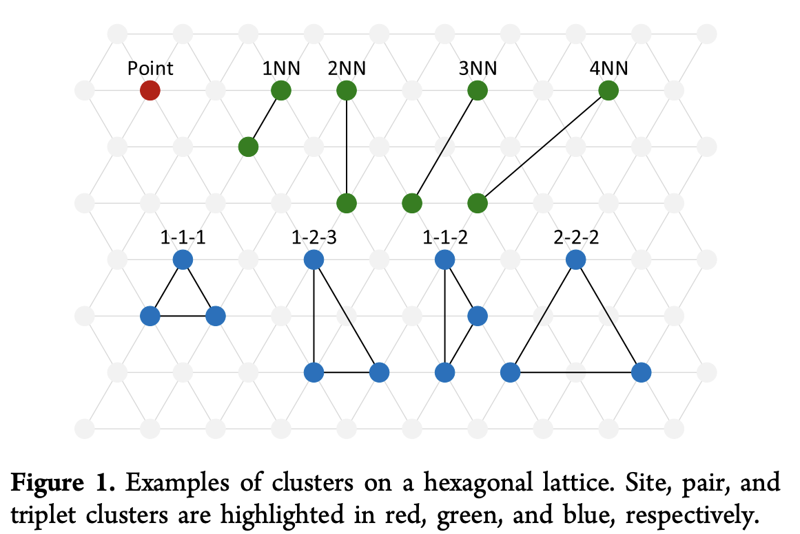
Given a set of clusters {\alpha}, the system’s Hamiltonian can then be rewritten as
E_{\textrm{CE}}(\sigma) = \sum_\alpha \sum_{(s)} V_\alpha^{(s)} \Phi_\alpha^{(s)}(\sigma) = V\Phi
Where E_{\textrm{CE}}(\sigma) is the energy per site of configuration \sigma, \alpha is the symmetrically distinct cluster, V_\alpha^{(s)} is the interaction energy of the of the cluster using the specified basis functions, \Phi_\alpha^{(s)} is the orbit averaged cluster function, V is the vector of interaction energies, and \Phi is the correlation matrix where rows correspond to configurations, and columns to symmetrically distinct clusters with different basis functions.
We’ve introduced a couple of new bits of terminology here, so let’s pause and explain. The new terms V_\alpha^{(s)} are analogous to the J terms in the previous expansion, and will be empirically fit (“learned”) from a dataset. The \Phi_\alpha^{(s)} are functions which map configurations \sigma to energy contributions. These are usually expressed as combinations of “basis functions”. We’ll see concrete examples of these for our Pt(111) system later in this post.
Part of the challenge facing cluster expansion is that there are a theoretically infinite number of configurations that can be sampled from the lattice. Which makes sense, since we’re selecting out a number of terms from the Taylor expansion to elaborate in more detail. In practice, the choice of clusters in the expansion ends up making a big difference in how accurate cluster expansion techniques are in practice. Past work has attempted to automated selection of clusters to expand by using genetic algorithms and other techniques like LASSO regularization. Another challenge is that cluster expansion tends to converge very slowly when adsorbates move away from ideal lattice positions and lateral interactions are nonlinear.
The authors note that convolutional methods tend to have strong predictive performance and have been applied for a number of materials property prediction tasks already. This authors suggest extending core graph convolutional techniques to prediction tasks on molecular lattices. At a high level, the intuition here is what if we can use a “lattice convolution” to make it so that we can make predictions directly from the lattice without having to select clusters for expansion at all. There’s a deep idea lurking here, that a convolutional network can serve to select an “automatic taylor expansion”. We’re moving a bit away from the core of the current paper, but I have a strong suspicion that this “automatic taylor expansion” property means that deep learning methods will have an even broader impact in computational physics over the next coming years.
Peeking ahead a bit, here’s a figure that lays out the core architecture of a lattice convolutional neural network (LCNN)
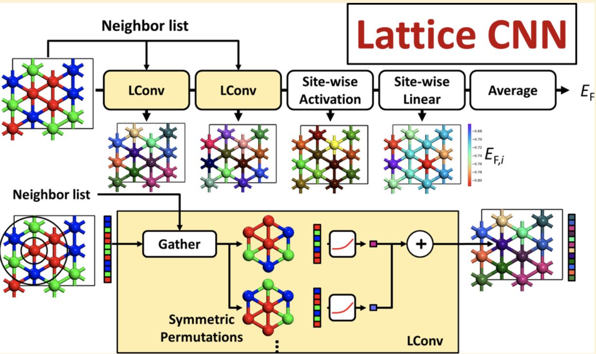
Notice how the raw lattice is directly fed into the algorithm! This has a powerful physical intuition in that we feed in the raw system without having to do an intermediate and somewhat arbitrary cluster processing technique.
Paper Summary
With that background primer out of the way, let’s dive into the actual contents of the paper.
As a brief summary, the authors benchmark their proposed new LCNN algorithm against various cluster expansion techniques (using manual heuristic and algorithmically guided cluster section). They also try using the convolution function from the recent crystal graph convolution paper. The work takes a stab at interpreting LCNNs by showing the model can decompose a system’s formation energy into individual site formation energies.
Pt(111) Benchmark Data
This paper only benchmarks on a single model system, the Pt(111) surface we discussed earlier. DFT values are pulled from an earlier study done on this system.
The test system that’s studied in particular here is the adsorption of \textrm{O}_2 on a \textrm{NO}-\textrm{O} equilibrated Pt(111) surface as we mentioned previously.
The formation energy for an adsorption configuration \sigma_i is denoted E_f(\sigma). The paper computes the formation energy as
E_f(\sigma) = \frac{E_f(\sigma) - E_0(0)}{N} - \frac{\theta_{\textrm{O}}}{2}E_{0,\textrm{O}_2} - \theta_{\textrm{NO}}E_{0,\textrm{NO}}
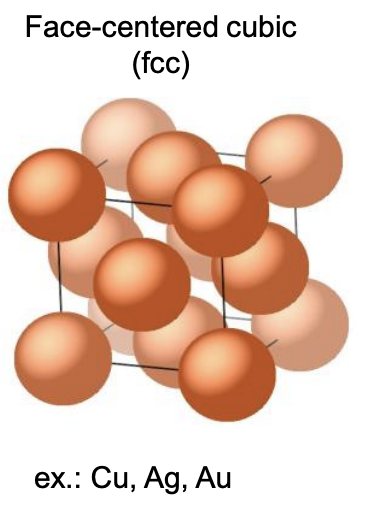
Where E_0(\sigma), E_0(0), E_{0,\textrm{O}_2}, and E_{0,\textrm{NO}} respectively are the DFT calculated electronic energies of configuration \sigma, the vanilla Pt(111) surface with no adsorbates, an oxygen molecule in vacuum, and a nitric oxide molecule in vacuum respectively. In addition, n_{\textrm{O}} and n_{\textrm{NO}} are the numbers of atomic oxygen and nitric oxide adsorbed, \theta_{\textrm{O}} and \theta_{\textrm{NO}} are the surface coverages of \textrm{O} and \textrm{NO}, and N is the number of fcc (face centered cubic) sites on the surface (image source).
The dataset in total has 653 configurations.
Cluster Expansion Implementation
This work uses networkX to computationally represent clusters. Nodes of the lattice graph contain site occupancy information, with 0 for vacant, 1 for \textrm{O} filled, 2 for \textrm{NO} filled. The following orthogonal basis set is used
\Theta_0(\sigma_i) = -\textrm{cos}\left ( \frac{2\pi\sigma_i}{3} \right )
\Theta_1(\sigma_i) = -\textrm{sin}\left ( \frac{2\pi\sigma_i}{3} \right )
Where \sigma_i is the occupancy of the i-th site, and \Theta_j is the j-th basis function. For a cluster in configuration \sigma, its weight is
\Phi_{a,i}^{(s)}(\sigma) = \Theta_{n_1}(\sigma_1)\dotsc \Theta_{n_{|a|}}(\sigma_{|a|})
Where \alpha is the cluster with lattice points {1,2,\dotsc,|a|}, (s) = {n_1,\dotsc,n_{|a|}} is the vector of indices indicating the basis function to use, and i is the index of a particular arrangement of the cluster in the configuration. Each element of correlation matrix \Phi corresponds to a configuration, cluster, and arrangement of basis functions and can be computed by
\Phi_{\alpha}^{(s)}(\sigma) = \frac{1}{N_{\alpha}^{(s)}(\sigma)} \sum_i^{N_\alpha^{(s)}(\sigma)} \Phi^{(s)}_{\alpha,i}
With N_{\alpha}^{(s)}(\sigma) the number of symmetrically distinct clusters in configuration \sigma. The following table shows an example of how to compute an element of the \Phi matrix
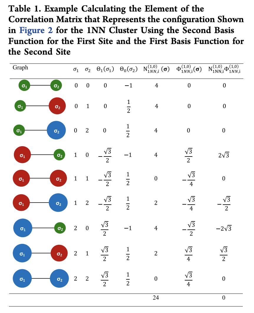
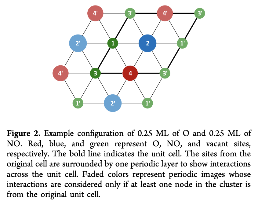
This calculation uses a hypothetical unit cells that’s displayed in the figure below:
Methods
Although the authors only consider Pt(111) as a benchmark system, they do a good job of benchmarking against a number of strong baseline algorithms
Heuristic Cluster Expansion
Clusters were selected using heuristic algorithms suggested in the literature. A linear model was used to determine the weights for each cluster using Scikit-Learn. 10-fold cross validation was used on the training set to select weights.
Genetic Algorithm Assisted Cluster Expansion
The authors used the ATAT to compute the genetic algorithm based expansion.
LASSO Assisted Cluster Expansion
The basic idea of the LASSO expansion is that the matrix V is encouraged to be sparse by addition of a L^1 penalty term. Mathematically, let C be a cost function, and \lambda the penalization hyperparameter. Then
C(\lambda) = \textrm{min}_V \|E_F - \Phi V\|^2_2 + \lambda \|V\|_1
\lambda is tuned via cross validation. The actual model is implemented using Scikit-Learn.
Lattice Convolutional Networks
The inputs for the lattice convolutional neural network are an atom feature vector A and an atom-pair feature vector P. Broadly, the LCNN formulation here follows that of the Weave convolutions from Google. Recall that Weave convolutions feature 4 different convolutional transformations, atom to atom A\to A, atom to bond A \to P, bond to atom P \to A, and bond to bond P \to P. As in other graph convolutional methods, atom descriptors are initialized with chemically relevant quantities such as atom type, chirality, formal charge, hybridization, hydrogen bonding, and aromaticity. Bond features include bond type, presence in the same ring, and spatial distance.
This current work adapts the original graph convolution framework to lattices by the following adaptations:
- Binding sites for adsorbates become nodes in the graph
- Edges represent immediately adjacent sites
The major challenge that faces lattices (unlike molecules) is symmetry. The core idea is that we want to consider multiple orderings of the neighbors of a given site so we have a symmetry-invariant local convolution. The following diagram illustrates the LCNN transformation:
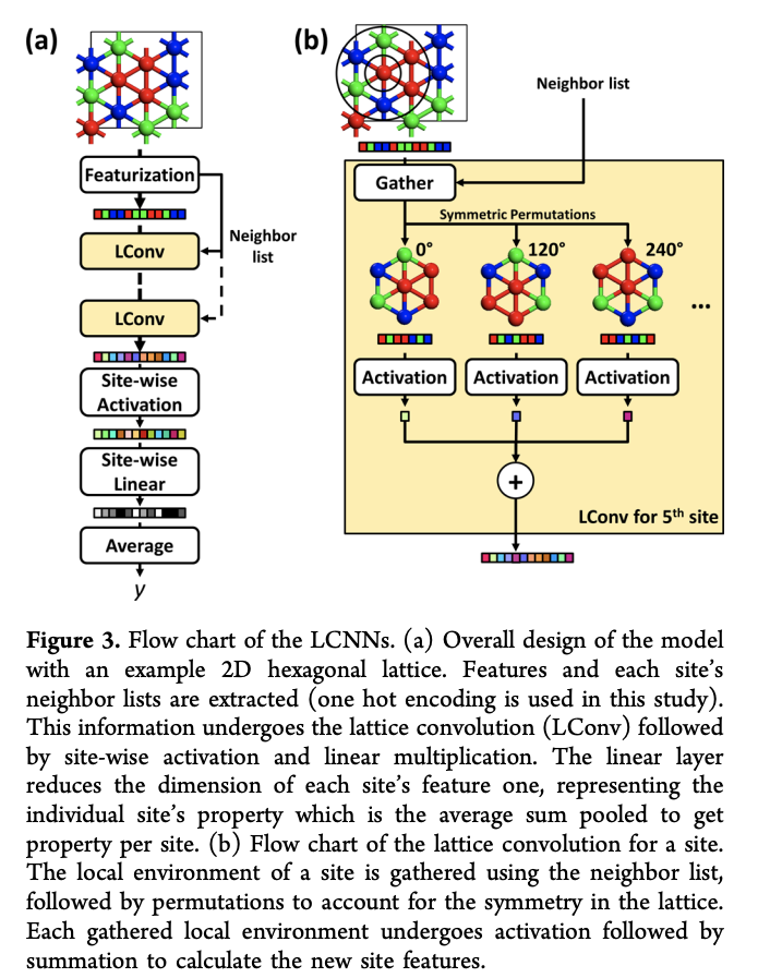
Let’s write down some equations. Given a periodic lattice with n_s number of sites, each site i has a site representation vector denoted x_i. This current paper simply uses one-hot encodings as the initial feature vector for each site, but it seems reasonable that more complex encodings could be used as well. After j convolutions have been applied, we denote the vector x_i^j. Let X^j = [x_1^j,\dotsc,x_{n_s}^j] denote the matrix of all binding site vectors after the j-th convolution. We can then formally write the LCNN convolution as
x_i^{j+1} = g(f(h(X^j, v_{i,1})), f(h(X^j, v_{i,2})), f(h(X^j, v_{i, 3})),\dotsc, f(h(X^j, v_{i,n_p}))
We’ve introduced a bit of new notation here so let’s unpack. Function h(X^j, v_{i,k}) gathers local environment around site i, where v_{i, k} is the k-th permutation considered. h(X^j, v_{i, k}) returns a subset of X^j in a given permutation order. f is the shifted softplus function. n_p is the number of different permuted orders of the neighbors that are considered in the convolution, and g is the summation function which “pools” the different permutations.
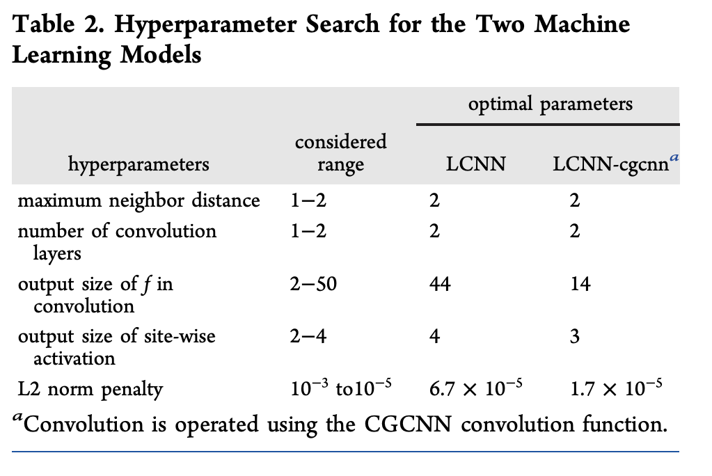
20 different choices of LCNN hyperparameters were tested. A variant of the LCNN, using the crystal graph convolutional loss function was also tested.
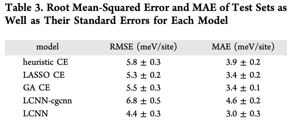
Evaluation Metrics
Models were evaluated with respect to root-mean-squared-error (RMSE) and mean-absolute-error (MAE):
\textrm{RMSE}_{\textrm{model}} = \sqrt{\frac{1}{N}\sum_i^N (E_{\textrm{model}}(\sigma_i) - E_F(\sigma_i))^2}
\textrm{MAE}_{\textrm{model}} = \frac{1}{N}\sum_i^N | E_{\textrm{model}}(\sigma_i) - E_F(\sigma_i)|
Here N is the number of test configurations, E_{\textrm{model}}(\sigma_i) and E_F(\sigma_i) are the formation energies of configuration \sigma_i predicted by the model and DFT respectively. Here are results from the various models:
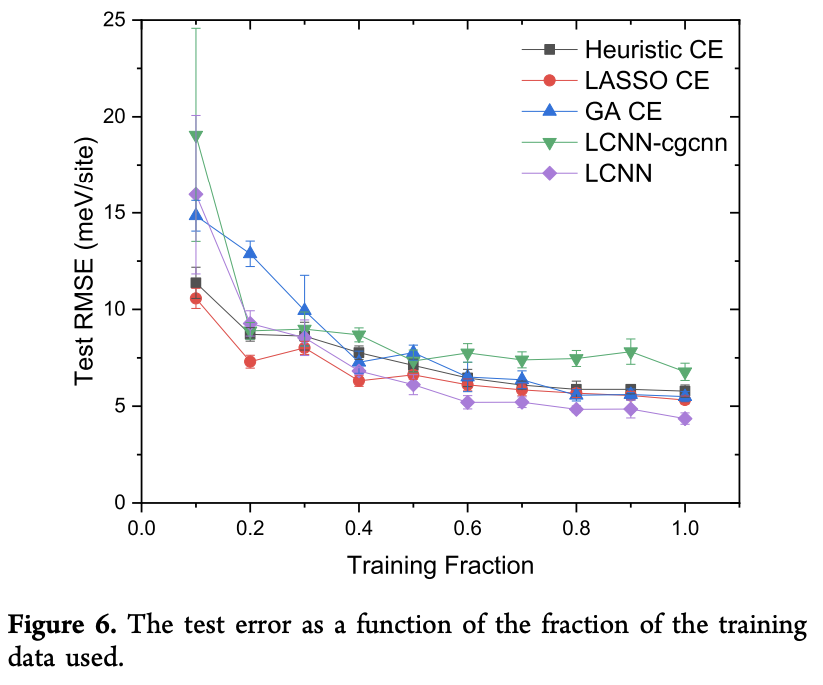
There was also a nice data efficiency experiment seeing how the various models trained on subsets of the data. Note how the LCNN model is about as data efficient as the other techniques, but achieves a lower final test error.
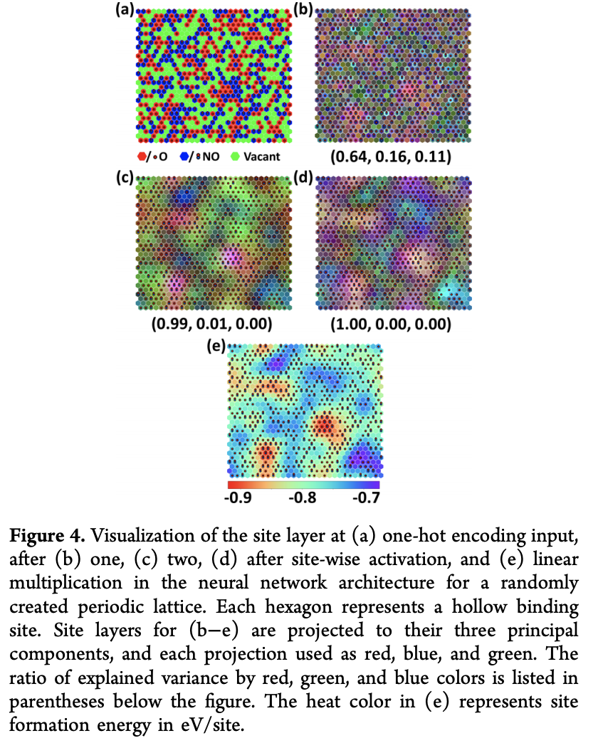
Visualizing the LCNN
The authors note that the site layers can provide a quick snapshot of what the model’s learned. The paper considers a 30x30 lattice, and randomly assings 270 \textrm{O} and 270 \textrm{NO} to sites. PCA is used to reduce representation vectors to 3 dimensions which are displayed as RGB. The figure below displays an intriguing sort of “spatial” averaging as it gets deeper.
Conclusion
Overall, this was an intriguing paper that extended the reach of graph convolutional methods to a new type of physical system. As with crystal graph convolutions, this paper extends the core mathematical structure of graph convolutions to handle more complex physical systems. I’m really excited to see where this line of work continues. Can graph convolutional systems handle complex fluid modeling for example?
One thing I’d have liked to see in this paper was evaluation on a test system that’s not Pt(111). The techniques here appear fairly general, but benchmarking a new technique is tricky. Until there’s additional information, it’s not clear that these techniques actually work better than the classical cluster expansion techniques.