I recently read the paper Mixture Descriptors toward the Development of Quantitative Structure–Property Relationship Models for the Flash Points of Organic Mixtures
Most physical descriptors are used to predict properties of single compounds. Most of the deep learning models in DeepChem and other packages are used for these applications. However many substances are not single compounds but rather mixtures. Fuel as used for cars is commonly a complex mixture of hydrocarbons for example. The literature around computational property prediction for mixtures is sparser than that for compounds though, so it was interesting to find this paper that described some computational modeling efforts on mixture data.
Mixtures can have complex physics, since the compounds that constitute the mixture interact with one another and each other in subtle ways. There are interesting effects such as azeotropic mixtures, which are mixtures that when boiling have vapor with the same fractional make-up as the original mixture. This means techniques such as fractional distillation can’t be used to separate out the constituents of the mixture. This is a curious sort of physical effect that demonstrates how a mixture can have interesting macroscopic physics that’s more than the sum of its parts.
The paper starts by noting that past work has suggested modeling binary mixtures by combining descriptors for the constituent compounds according to their mole fractions. Such models have been used to predict things like the densities and infinite dilution activity quotients of binary mixtures. Other work has tried to predict things like the boiling points of azeotropic binary mixtures.
This paper focuses on the challenge of predicting the flash points of mixtures. The flash point is the temperature of vapor ignition above a volatile liquid. Being able to predict the flash point would be Important for safety while experimenting with new mixtures especially when working with petrochemicals. Past work has attempted to build predictive models for flash point prediction, with one model achieving 2.5 Celsius mean average error (MAE) for a dataset of 1K pure compounds
How then can you predict the flash point of mixtures? The paper explains that the usual technique is to use “mixing rules” for predicting flashpoints. The authors note that a recent paper used a mole-fraction weighted average values of mixture descriptors along with a genetic algorithm and multilinear regression to make the actual prediction. The authors broadly follow a similar approach.
Dataset Description
A dataset of 435 experimental flash points for both pure compounds and mixtures was gathered from 13 references in the literature. Here’s a diagram of the distribution of flash points ins the source data
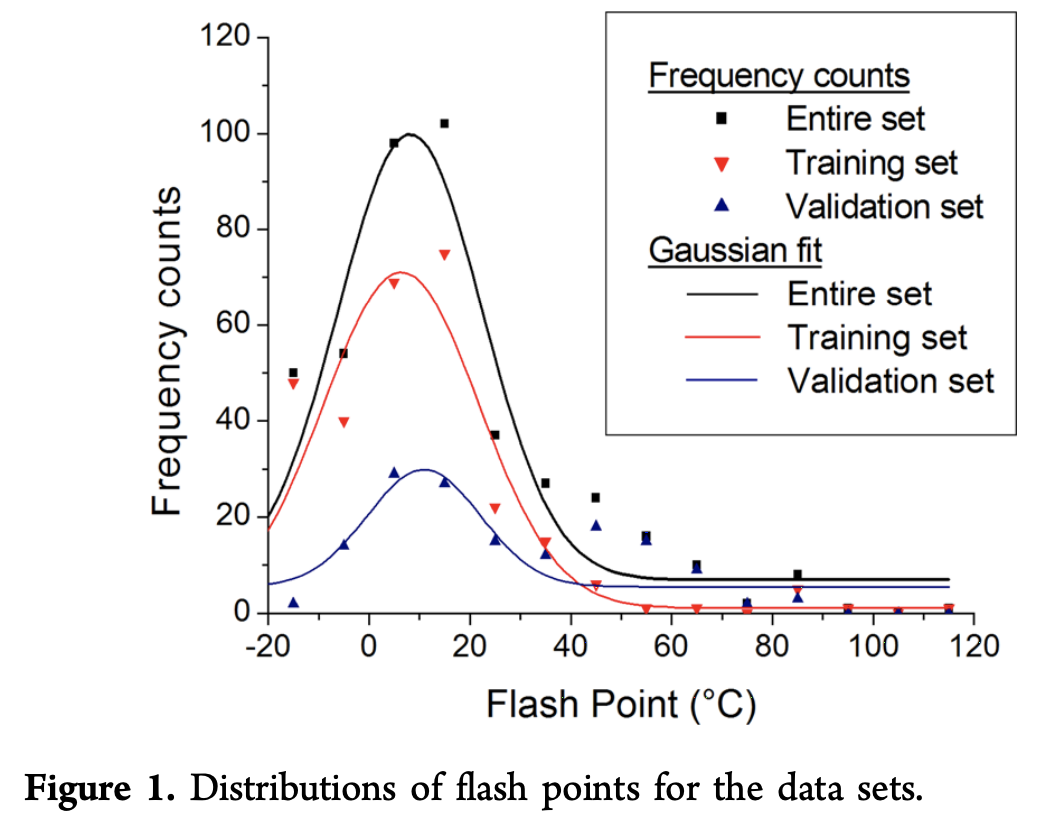
Some effort was taken to ensure that the validation set and the training set had different distributions. Training set compounds had flash points measured according to the ASTM D56 standard, while validation compounds had those measured according to REACH standards
Compound Descriptors
Descriptors were computed by using Gaussian to compute DFT calculations to obtain low energy structure. 300 molecular descriptors were computed from these structures. These were split into 4 categories of descriptors
- Constitutional descriptors: identification and count of specific features of the molecule
- Topological descriptors: descriptions of the 2D structure of the molecule.
- Geometric descriptors: descriptions of the 3D shape of the molecule
- Quantum chemical descriptors: binding, energetic, electronic, thermodynamic information
Descriptors were computed from the DFT generated structures using Codessa.
Mixture Descriptors
Mixture descriptors D were computed by taking molecular descriptors d_i of each component, taking into account their respective mole fractions x_i.
D = f(d_i, x_i)
The authors note that the flash point of mixtures isn’t a simple linear combination effect of the substituent elements. Rather, there are more complex interactions between compounds like their affinities and respective vapor pressures. This work tests 12 different simple mathematical formulas for f, with 5 extracted from the literature and 7 they’ve introduced. The authors divide their proposed formulas into 3 classes
Direct Combinations
All of these proposed formulas are symmetric with respect to molecular descriptors and mole fractions. Mathematically put, that means
D = f(d_1, x_1, d_2, x_2) = f(d_2, x_2, d_1, x_1)
A second sanity property is that if the mole fraction of one compound drops to zero, the descriptor shouldn’t depend on that compound. Stated in equations
D = f(d_2, x_2) \textrm{ if } x_1 = 0
The simplest formula \textrm{fmol_sum} is a weighted linear combination. (The paper introduces simple names like \textrm{fmol_sum} to track the various formulas at hand.)
D = x_1 d_1 + x_2 d_2
An alternate is the weighted absolute difference \textrm{fmol_diff}
D = | x_1 d_1 - x_2 d_2|
Other variants are the square mole fraction \textrm{sqr_mol} and square-root mole fraction \textrm{root_fmol}
D = x_1^2 d_1 + x_2^2 d_2
D = \sqrt{x_1} d_1 + \sqrt{x_2} d_2
Another alternatives are the square molar contribution \textrm{sqr_fmol_sum} and the norm of the molar contribution \textrm{norm_cont}
D = (x_1 d_1 + x_2 d_2)^2
D = \sqrt{(x_1d_2)^2 + (x_2 d_2)^2}
Deviation Combinations
These combinations depend on the differences \Delta d = |d_2 - d_1| and \Delta x = |x_2 - x_1|. The first deviation combination they consider is \textrm{mol_dev}
D = (1 - \Delta x) \Delta d
Here are two other variants respectively called \textrm{sqr_mol_dev} and \textrm{mol_dev_sqr}.
D = (1 - (\Delta x)^2) \Delta d
D = (1 - \Delta x)^2 \Delta d
Other Combinations
Here are some other variant contribution formulas that they consider. \textrm{cent} computes the centroid
D = \frac{\sum_i d_i}{n}
Where n is the number of compounds in the mixture. Two other formulas are \textrm{sqr_diff} and \textrm{abs_diff}
D = (d_1 - d_2)^2
D = |d_1 - d_2|
Models Considered
This work trains simple multilinear regression models such as
Y = \sum_i a_i D_i + a_0
Where D_i are the mixture descriptors. A heuristic pruning method was used to prevent overparameterization and ensure that the multilinear regression didn’t have too many terms. I wonder why the authors didn’t use techniques like LASSO, but perhaps it’s because they wanted to extract interpretable formulas easily (which they do later in the paper).
Model Performance
All mixtures in the validation set were constituted with at least one pure compound that wasn’t in the training set. Here’s some error calculations with different choice of formula f
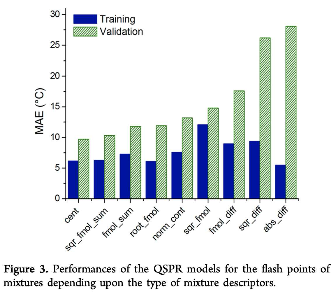
The centroid \textrm{cent} seems to work well empirically, but an important point to note about the centroid equation is that it is aphysical since it doesn’t use information provided by the mole fractions x_i. To make this point clear, the paper considers a variety of 4-methyl-2-pentanone/1-butanol mixtures in different proportions
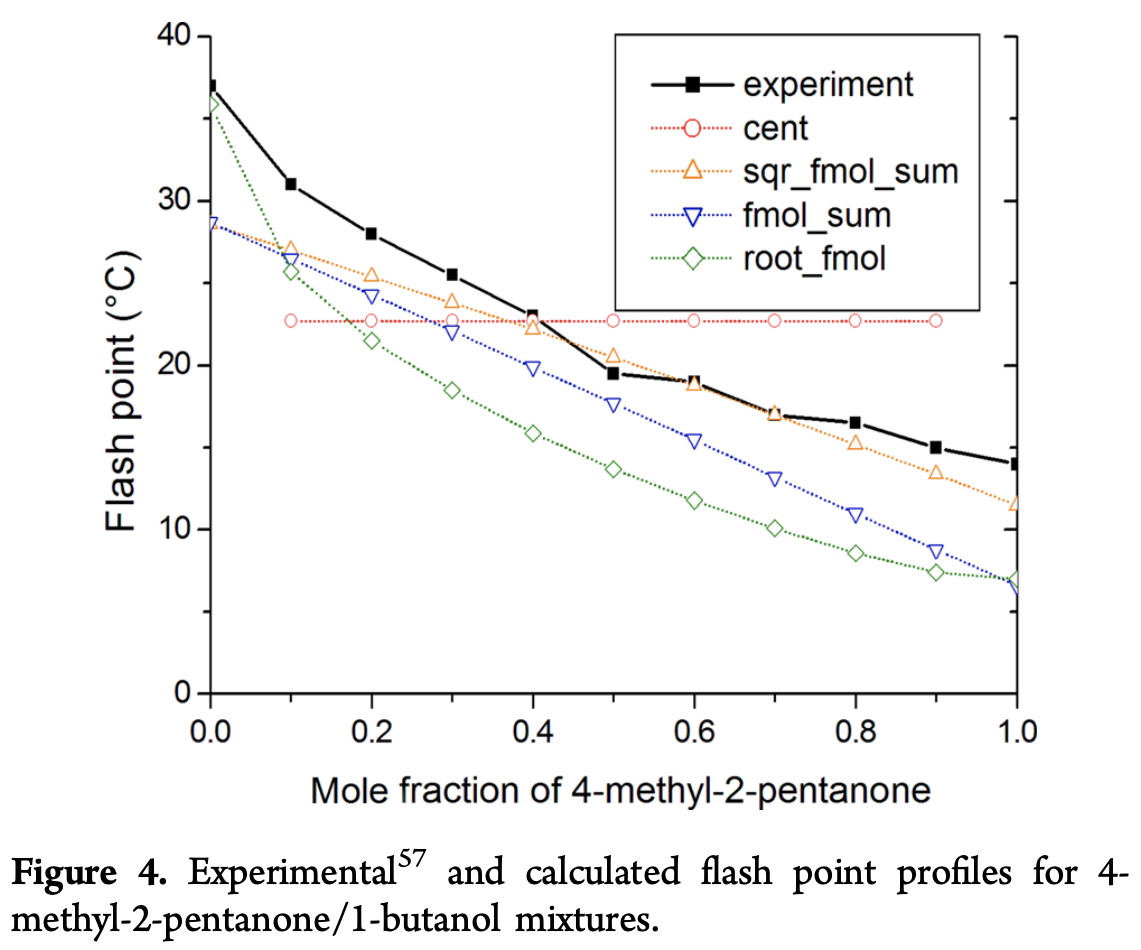
Note how the \textrm{cent} line shows no sensitivity to this alteration. To gauge generalizability of various formulas for f, the paper considers different classes of mixtures and sees how well different choices for f do.
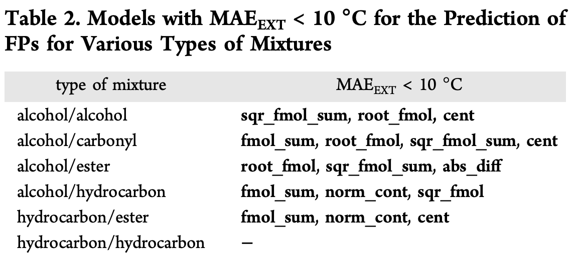
The weighted linear combination \textrm{fmol_sum} seems to do well across many categories. However, they note that this simple weighted sum does poorly at predicting the behavior of non-ideal mixtures that have very nonlinear interaction effects. They show an example on a 1-propanol/octane mixture:
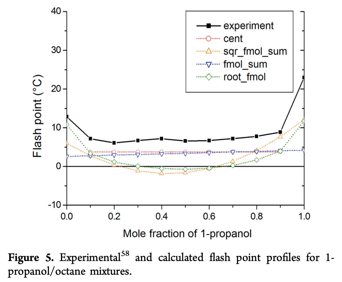
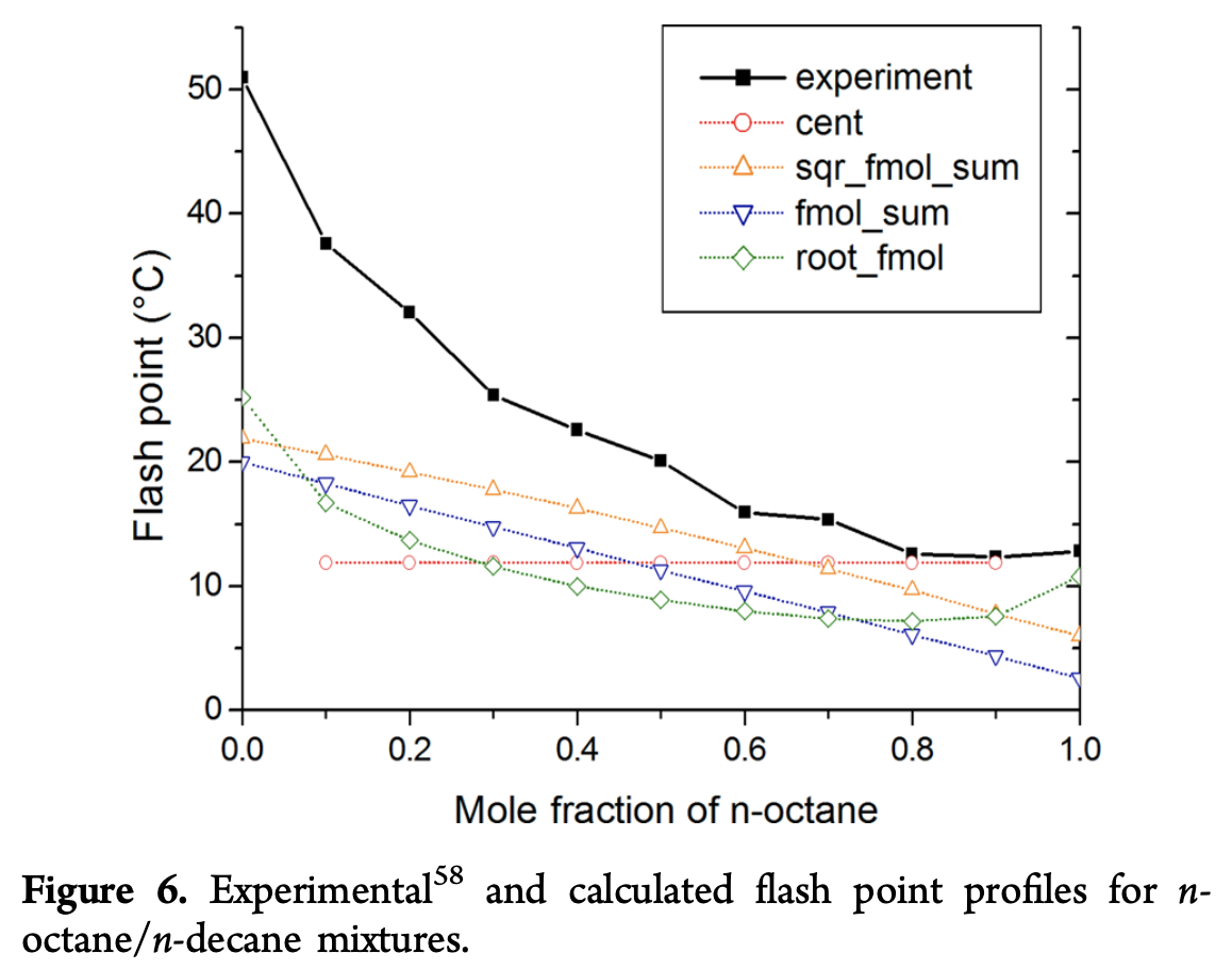
This mixture is especially dangerous since the flash point lowers for mixtures, which means that the mixture is more dangerous to handle than either of the constituent compounds which could prove very dangerous for experimenters. As a general note, all models don’t seem to do well at the extremes of predicting behavior of pure compounds. This issue is particularly clear in the figure below analyzing n-octane/n-decane mixtures, where there are errors on the order of 25 C.
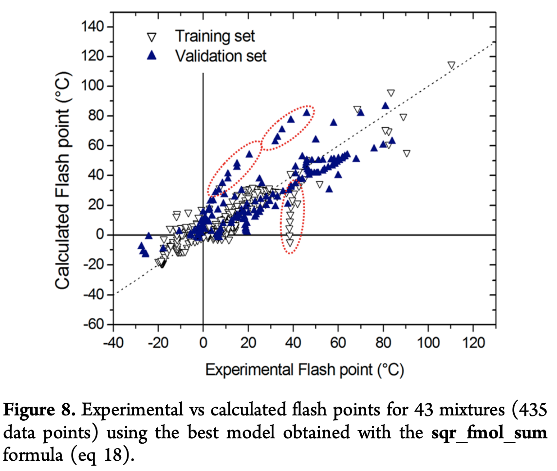
Interestingly, one step the authors do is to pull out the best performing model overall and extract the actual formula it computes. Their heuristic method for multilinear regression yields a formula with a limited number of terms. This provides the following equation for flash point prediction from a collection of simpler material properties.

Here, \textrm{FP} is the flash point, x the mole fraction, {}^3\chi_1 is a “Randic index”, a type of topological descriptor of a molecule, \textrm{HDCA2} the Hydrogen donor charged surface area, \Delta \alpha the anisotropic polarizibility, and V_{\textrm{min},H} the minimum valency of a \textrm{H} atom. They then plot how this best model does on the validation set
Discussion
Although the authors don’t directly say so in the work, it feels like a lot of this work was motivated by the needs of the petrochemical industry. The choice of flashpoint as the core property to study (of high importance when considering fuel mixtures) and the multiple figures that involve hydrocarbons make this pretty clear.
The biggest comment I have on this work of course is that the models chosen here are pretty simple linear models. I suspect it would be feasible to re-use the analysis of various mixture formulas here, but to use a deep learned featurization for the mixture components. This learnable architecture may be easier to generalize to other classes of mixtures, say for electrolytes in batteries. In addition, the addition of learnable nonlinearities may enable models to handle the edge conditions that the linear models in this paper struggled with. The biggest challenge with this idea is likely that not enough data is available to train more general models. I think that effective use of transfer learning or other strong priors will be necessary to make these models broadly applicable.
This paper goes deeper into industrial chemistry than my usual reading. But I think there’s an important point here that deep learning doesn’t yet seem to have made major inroads into understanding the physics of complex materials such as mixtures. This seems only a matter of time though, so it’ll be interesting to see how this field progresses.

