I recently read the paper Deciphering interaction fingerprints from protein molecular surfaces. The code for this paper is available at https://github.com/lpdi-epfl/masif.
The paper introduces a new framework MaSIF (Molecular Surface Interaction Fingerprinting) for extracting descriptive “fingerprints” from protein structures for use in applications such as protein-pocket/ligand prediction, protein-protein interaction site prediction, and fast scanning of protein surfaces for prediction of protein-protein complexes.
The introduction makes the point that there are multiple types of evolutionarily conserved behavior in proteins. Most bioinformatic techniques depend on sequence homology to infer similar behavior. However, in many cases, the conserved structure may be the behavior of the “molecular surface.” It’s possible for proteins with low sequence homology to exhibit very similar biochemical behavior due to surface similarity. This paper proposes that geometric deep learning methods could perhaps be used to extract these surface fingerprints automatically. The authors hypothesize that proteins with no sequence homology may have similar surface interaction patterns, especially if they serve similar biochemical purposes. This means that extracted fingerprints could be used to answer non obvious questions about protein behavior, in niches where evolutionary methods could fail.
As a bit of side note, what defines a “molecular surface”? It really comes down to solvent accessibility. What parts of the protein are accessible to solvents in folded state. Note that knowledge of the molecular surface has to currently be extracted from experimental crystallography data (and perhaps cryo-EM data). At present, it isn’t really feasible for the surface to be predicted from sequence directly, since you’d need to be able to computationally fold the protein to make this prediction. This could perhaps change over the next 5 years as techniques like AlphaFold mature.
The core idea of the MaSIF approach is to decompose a surface into a collection of overlapping radial patches with fixed geodesic radius. A descriptor is then computed for each patch, encoding a description of the features present in the patch. These local descriptors are then passed through a series of convolutional layers to the downstream loss function. The figure below lays out the core ideas in this framework.
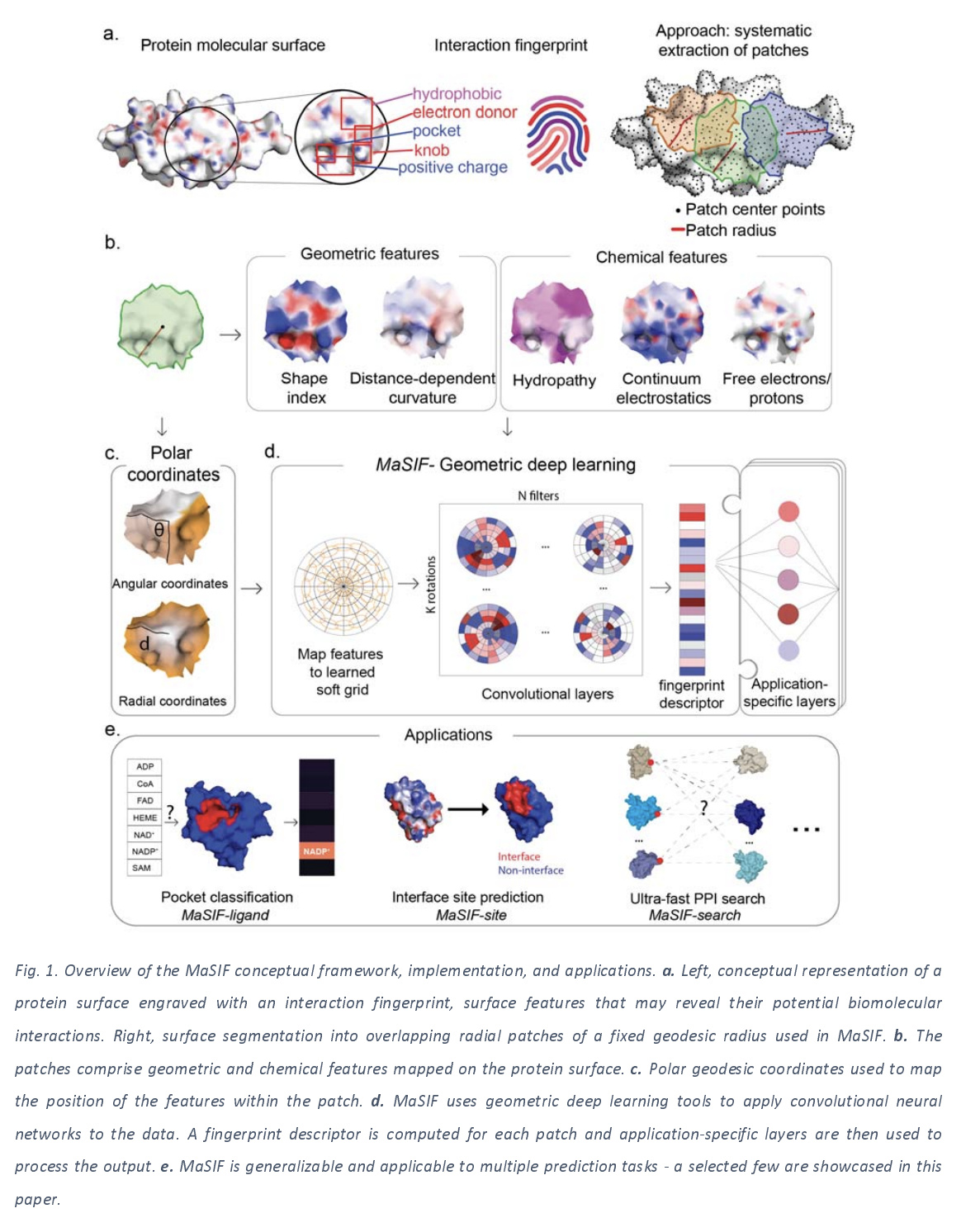
Here’s a rough overview of the MaSIF framework. An input PDB file (recall that a PDB file holds a 3D structure for a biomolecule such as a protein) is taken in and processed. This process involves cleanup, protonation (adding hydrogens correctly to provide a representative state for the Ph of the molecule), and a couple other steps.
This molecular structure is then discretized as a mesh, based on the solvent excluded structure. Each vertex in this new mesh is tagged with a number of local descriptors which provide information about the local shape and chemistry at that vertex on the surface. The mesh is then broken into a collection of local patches, with a geodesic radius of either 9 or 12 angstroms. Vertices within a patch are then converted into polar coordinates (with respect to the center of the patch), then fed into a learnable kernel which averages the per-vertex feature vectors into a patch vector. The paper refers to this learned transformation as a learned soft grid. One subtlety here is that for each patch, there’s no canonical axis to compute angles from, so each patch has a randomly sampled axis. In order to average out this dependence on a random axis, the authors perform K rotations on the patch, and max-pool the output to get a rotation invariant learned kernel. This procedure provides a local patch vector (the paper calls this a surface fingerprint) for a collection of overlapping patches on the surface. These patches are then combined in some fashion to produce the final output. (The combination method depends on the exact downstream architecture)
These molecular surfaces are then fed into a geometric deep learning architecture. Such geometric deep learning techniques try to generalize core convolutional architectures to other geometries including surfaces, graphs, and even arbitrary manifolds. In this work, the authors focus on processing local extracted patches with their techniques, but at a high level, this approach is pretty similar to techniques such as graph convolutions or atomic convolutions.
One important thing to note is that MaSIF isn’t one deep architecture. Rather, it’s a collection of ideas for constructing deep architectures that work directly from protein structures. For this reason, there’s a lot of technical details involved in actually implementing the algorithms discussed in this work. The authors github repo is an excellent resource with details and code for all the transformations performed. I’ll try to provide an overview of the core ideas in this post, but I’ll have to refer readers to the paper and repo for the full details.
In the remainder of this post, I’ll review some of the applications the authors consider. Namely, ligand prediction for protein binding pockets, site prediction in protein-protein-interactions, and fast scanning of molecular surfaces to predict the structural configuration of protein-protein complexes. But before we get to applications, let’s do a quick deep dive on the actual features computed for each patch, and a bit of the math used for learned soft grids.
Preparing Protein Structures
Protein structures from the PDB were protonated with Reduce. Meshes were triangulated using MSMS. Meshes were downsampled and regularized using Pymesh
Computing Feature Vectors
A number of local features were computed for each patch:
- Shape Index: This is computed in terms of the principal curvatures \kappa_1, \kappa_2 and is defined as
\frac{2}{\pi}\textrm{tan}^{-1}\frac{\kappa_1+\kappa_2}{\kappa_1 - \kappa_2}
- Distance Dependent Curvature: For each vertex within a patch, this computes a type of local curvature, based on techniques from the paper Fast screening of protein surfaces using geometric invariant fingerprints.
- Poisson Boltzmann continuum Electrostatics: This used the PDB2PQR utility (https://github.com/Electrostatics/apbs-pdb2pqr) to compute Poisson-Boltzmann electrostatics for each protein.
- Free Proteins and Electron Donors: The location of free electrons and potential hydrogen bond donors in the patch was computed. Then a value was from a Gaussian distribution was attached to each vertex ranging from -1 (optimal hydrogen bond acceptor) to +1 (optimal hydrogen bond donor). This technique was adapted from the paper An orientation-dependent hydrogen bonding potential improves prediction of specificity and structure for proteins and protein-protein complexes
- Hydropathy: Each vertex was given a hydropathy score, ranging from -1 (hydrophilic) to 1 (hydrophobic).
Angular Coordinates
After local patches are constructed, MaSIF uses a geodesic polar coordinate system to specify the positions of vertices in each patch to radial/angular coordinates with respect to the center of each patch. The Djikstra algorithm was used to compute an approximation to geodesic distance, and a multidimensional scaling algorithm implemented in matlab was used to compute local angular coordinates. The github repo attached to this paper has swapped to using Python in its latest release, but the original matlab code is also available.
Geometric Deep Learning
The actual learning uses a technique adapted from Geometric Deep Learning on Graphs and Manifolds Using Mixture Model CNNs. The surface patch is mapped to a “soft learned” 2D polar grid, and then a series of convolutional layers are applied. The continuous patch is discretized into \theta angular bins and \rho polar bins for a total of J = \rho\theta bins. Let x be a vertex in the discretized grid, then let N(x) denote its grid neighbors. If y \in N(x), then let u(x,y) denote the radial/angular coordinates of y with respect to x. Let f(y) be the feature vector at y, and let w_j be a weight function, Then the convolution operation is defined as
D_j(x) f = \sum_{y \in N(x)} w_j(u(x,y))f(y), \quad \quad j = 1,\dotsc,J
To implement rotational invariance, \theta rotations of the input patch are performed, and a max pooling layer is used to sum contributions
Ligand Prediction for Protein Binding Pockets
With that background material out of the way, let’s return to considering applications. The first one the paper considers is that of predicting the behavior of protein binding pockets.
The authors motivate their focus on protein binding pockets by noting that interactions between proteins and small molecule metabolites is very important for understanding homeostasis, but is something that’s poorly understood. They hypothesize that an interaction fingerprint extracted from each binding pocket could be used to predict metabolite binding preference, and focus on seven metabolites (NADP, NAD, HEME, FAD, CoA, SAM, ADP) for their study. The next figure lays out their core results for this task.
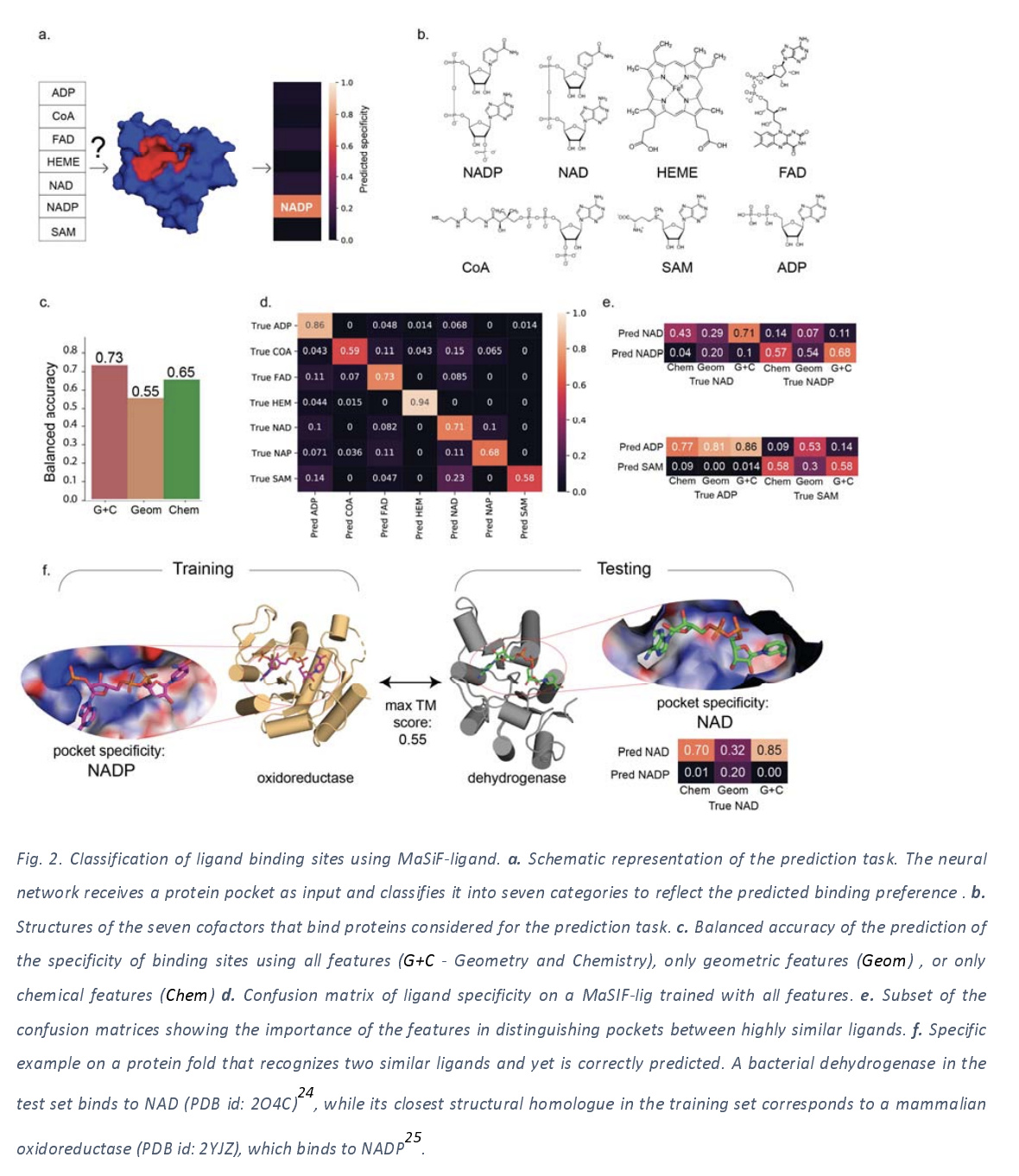
The binding site model is trained using a collection of cofactor binding proteins extracted from the literature, with the training and test sets separated by sequence clustering to make sure that the test set wasn’t too like training. A random model would be expected to have about 14% balanced accuracy, but their trained models achieve 73%, showing a strong ability to predict metabolite binding preference from binding site structure.
One thing that this application makes me curious about is how well this system would work for predicting binding affinity for arbitrary ligands. The authors note that performance is variable across the different metabolites, with HEME doing well, perhaps because it’s very distinct from the other ligands and easy to identify. I bet this architecture could be combined with a graph convolution for the ligand molecule, leading to improved performance, and I’m reasonably sure some papers exploring similar ideas have come out already.
Binding Pocket Training Data
Data to train on was pulled from the PDB (Oct 16, 2018), with all structures that included a protein chain, but not structures that included DNA/RNA. Sequence similarity was used to further separate the training dataset from the validation dataset. In total, 1459 structures were used, with 72% training, 8% validation, 20% testing.
Binding Pocket Neural Network Architecture
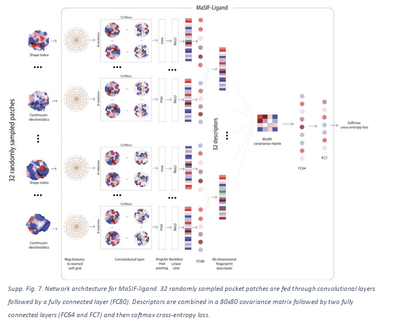
Let’s do a quick deep dive on the actual architecture used. 32 patches were sampled from each binding pocket. Each patch was used as an input into a network and mapped to a learned soft grid. Patches were transformed into 80 dimensional feature vectors, then feature vectors were multiplied together to create a 80x80 covariance matrix, which was then passed through additional fully connected layers which fed into a cross entropy loss function.
For stable predictions, each pocket was sampled 100 times, and the 100 predictions were averaged for the final prediction.
Predicting Protein Binding Sites from Interaction Fingerprints
The next task the authors take on is the challenge of taking a particular protein surface and outputting a score that estimates the likelihood of that surface being involved in a protein-protein interaction. The next figure lays out the results of their architecture applied to this task.
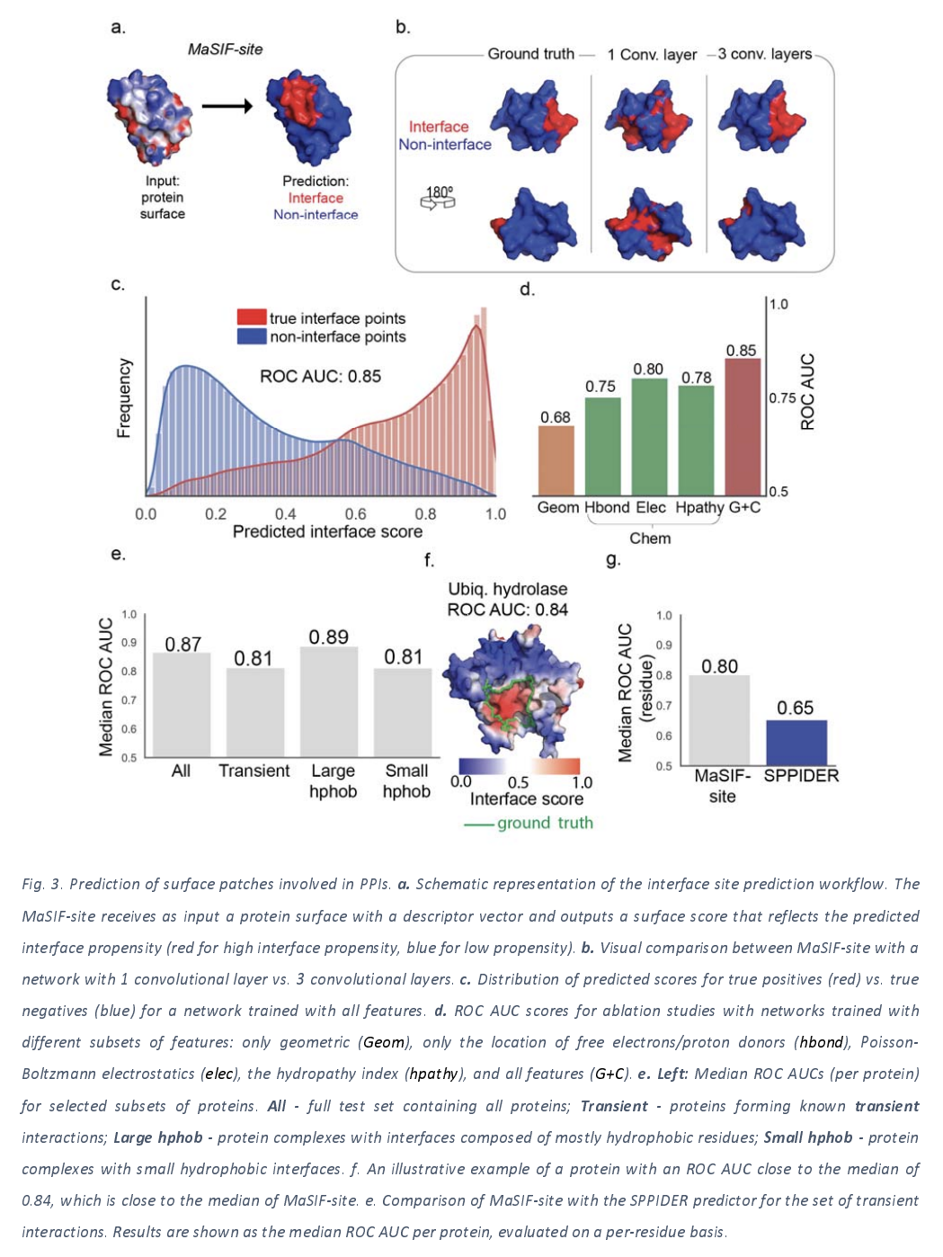
An interesting thing to note is that the depth of the convolution applied seems to make a difference for this application, with 3 layer deep networks performing better than shallower networks. Interestingly, the deep approach also provides a nice performance boost over simpler alternative approaches such as SPPIDER.
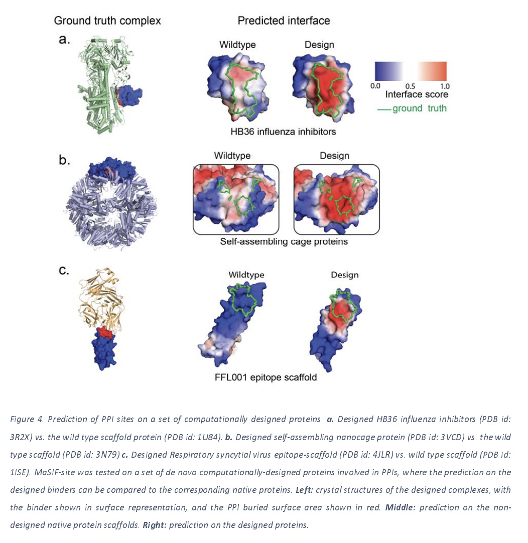
The authors note that there’s been a lot of progress in de novo design of proteins in the last few years, and that the binding sites for designed proteins can’t be inferred from evolutionary information. However, it looks like MaSIF techniques can do decently at this task as this next figure illustrates.
Protein-Protein Interaction Training Data
For protein-protein-interaction data, the PRISM database (a compendium of PPIs found in crystal structure data) was used as the original datasource. This database was filtered for PPIs that don’t have a minimal degree of interaction. 8466 proteins were pulled from PRISM. Other PPI structures were pulled from PDBBind, SAbDab, and ZDock. The total 12002 proteins were clustered using psi-cd-hit (a package for comparing protein sequences) into clusters, and one representative example was selected from each cluster. This resulted in 3362 proteins which were split into training and validation.
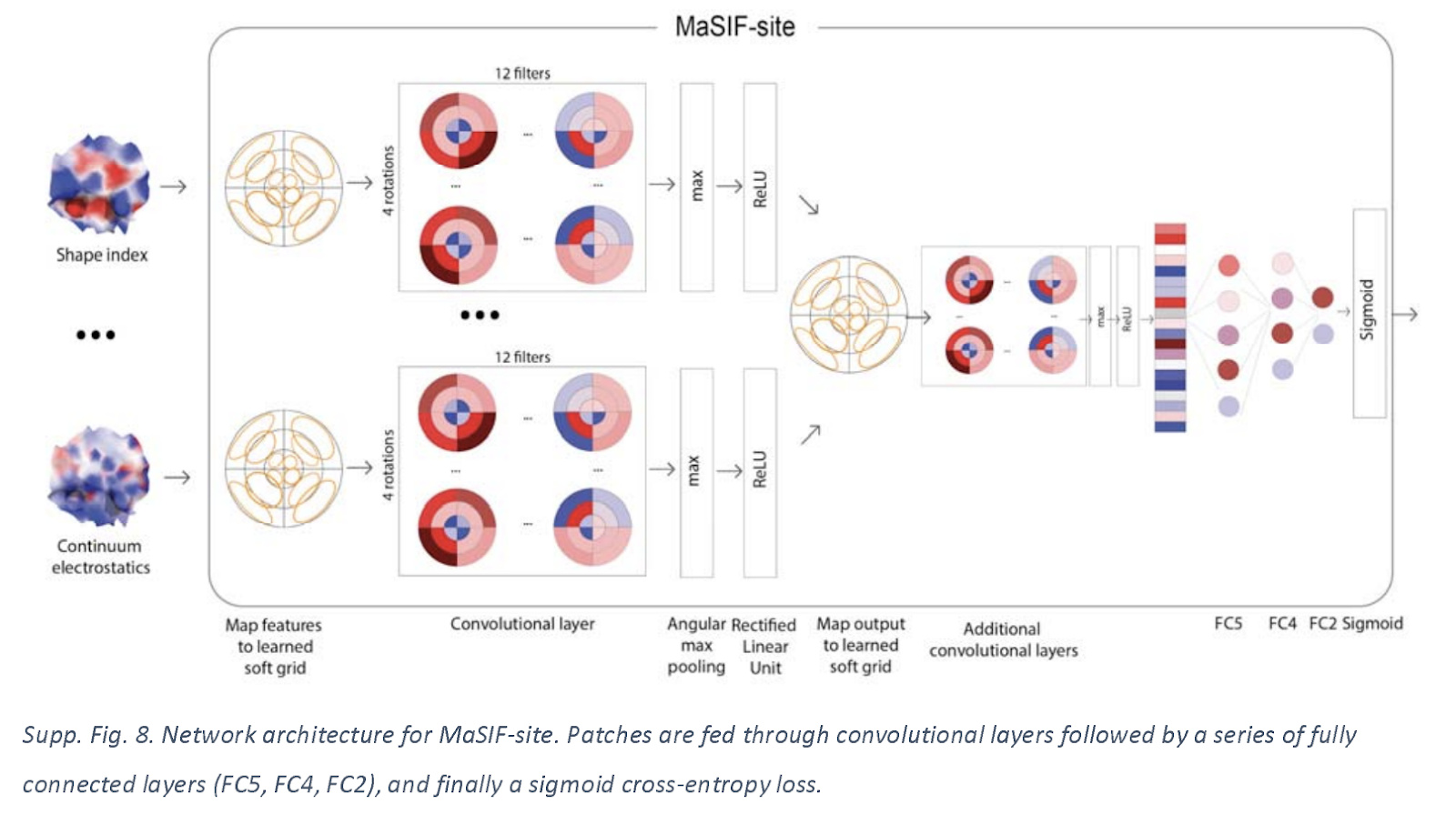
Site Prediction Neural Architecture
Let’s take a quick look at the architecture used for this application. The network receives a full protein decomposed into a set of overlapping surface patches with radius 9.0 angstrom. These patches are mapped onto learned grids with 3 radial bins and 4 angular bins.
Fast Scanning of interaction fingerprints for predicting protein protein complexes
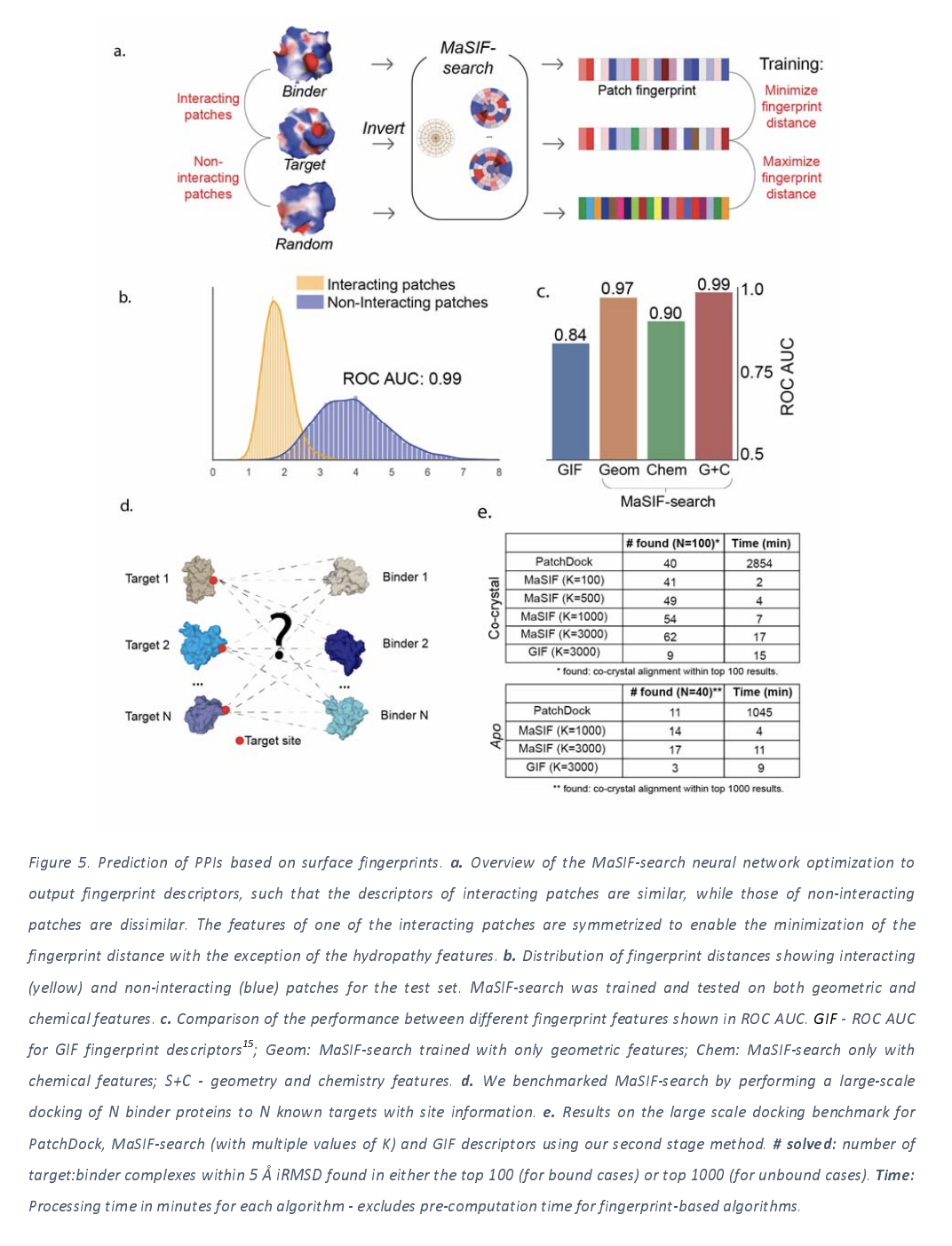
This last application takes the interaction site prediction of the previous application one step further. The basic idea is that if you can compute fingerprints for two proteins and use the fingerprints to predict whether or not two proteins will interact. This idea is compelling since predicting protein-protein interaction through docking is very slow, so being able to use a rough deep learning approximator could speed up applications considerably.
The work makes the assumption that two protein patches will interact if they have complementary surface patches with complementary geometric and chemical features. This model is trained with a database of 100K interacting protein patches they extract from structural databanks, along with randomly sampled negatives. The trained model achieves quite high accuracy at its task as the figure below shows.
PPI search training data
The PRISM database was used as in the previous application. Hierarchical clustering was used to separate proteins in the training and test sets apart from one another. Positive pairs of patches were extracted as two patches within 1.0 angstrom of one another. A radial shape complementarity score was computed for each pair. 85652 true patches and 85652 random patches were used for training. 12678 true and 12768 random patches were used for testing.
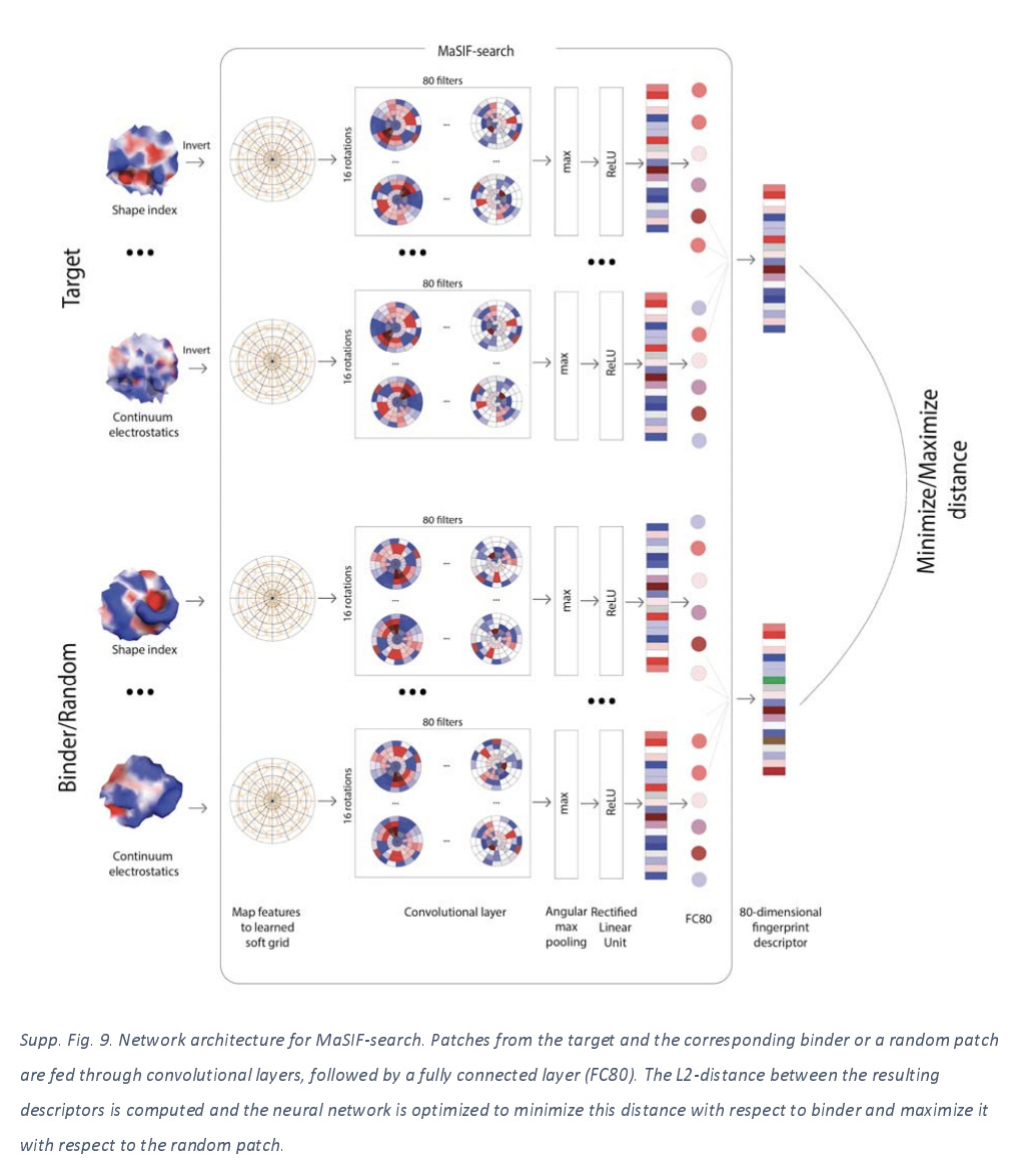
PPI Search Neural Architecture
Let’s take a quick peek at the architecture used for search. Notice how this architecture takes in targets paired with either binding or random patches. The network was trained to minimize the Euclidean distance of true binding pairs and maximize the Euclidean distance of nonbinding pairs.
Some Concluding Thoughts
I really liked this paper. It pulls together a host of ideas from bioinformatics, physical chemistry, and deep learning to provide a compelling framework for answering biophysical questions about proteins. The only drawback I see to this paper and approach is that there’s a lot of different details that need to be handled correctly for this approach to work out. The authors have put out good open source code which will help reproduce their work, but I suspect a lot more heavy lifting will need to happen before these techniques are widely usable.
